How To Freeze Rows Or Columns In Excel Sheets:- Let’s say you have a really long excel sheet. The first row contains the names of all the columns and is being used by you as a reference to enter values. You are entering values row by row into the Excel sheet. As the number of rows increases, you will not be able to see the first row which is used a reference. In that case, you might want to freeze your first row for better utilization of time and effort. This article deals with exactly that. Read on, to learn how to freeze rows or columns in Excel sheets.
How To Freeze Rows In Excel Sheets
STEP 1
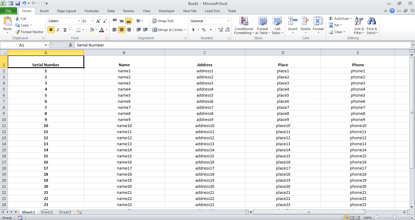
- Let’s see what’s wrong and what can be done to fix it. Open your really long sheet in Excel.
STEP 2
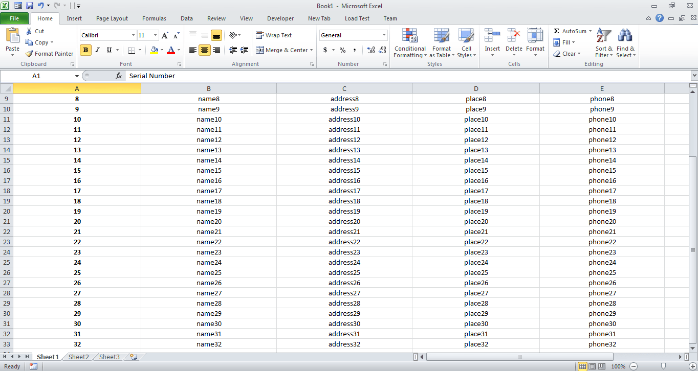
- Scroll down. Now as you can see, the first row that contained the column names like Serial Number, Name, Address etc is scrolled up. Right now, we are unable to figure out the column names. The only way is scrolling up and finding out. But if your Excel sheet is really really long, this definitely wouldn’t be a feasible solution. Follow the steps below for an easy solution.
STEP 3
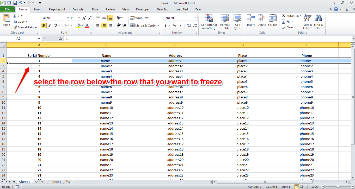
- Let’s say you want to freeze the first row. That is, the row that contains the column names. In that case, you have to select the row just below the first row.
STEP 4
- Once you have selected the entire row, click on the tab View. There will be a button named Freeze Panes under the View tab. Click on the drop down arrow associated with it to find and click on the option named Freeze Panes. If you have already frozen your panes, then this option will be Unfreeze Panes. You can choose as per your choice.
STEP 5
- Viola! Now if you scroll down, you can see that the row that you wanted frozen is actually frozen!
How To Freeze Columns In Excel Sheets
STEP 1
- If you scroll horizontally, the fields in the left will get moved to the left. What if you want to see the filed at the very left to be always visible?
STEP 2
- In that case, select the column next to the column that you want to freeze. Once you have selected the column, click on the View tab as before. Find the button Freeze Panes. Again, click on the option Freeze Panes from the drop down menu.
STEP 3
- Now if you scroll horizontally, you can see that the left most column, that is the Serial Number column is fixed.
You can’t freeze a particular row or column from somewhere in the middle using this feature. If you freeze a row or column, all the rows or columns above or before it will be frozen. Hope you found the article useful. Stay tuned for more tricks, tips and hacks.


